Tree data structures have many uses, and it’s good to have a basic understanding of how they work. Trees are the basis for other very used data structures like Maps and Sets. Also, they are used on databases to perform quick searches. The HTML DOM uses a tree data structure to represents the hierarchy of elements. This post will explore the different types of trees like binary trees, binary search trees, and how to implement them.
We explored Graph data structures in the previous post, which are a generalized case of trees. Let’s get started learning what tree data structures are!
This post is part of a tutorial series:
Learning Data Structures and Algorithms (DSA) for Beginners
Trees Data Structures for Beginners 👈 you are here
Trees: basic concepts
A tree is a data structure where a node can have zero or more children. Each node contains a value. Like graphs, the connection between nodes is called edges. A tree is a type of graph, but not all graphs are trees (more on that later).
These data structures are called “trees” because the data structure resembles a tree 🌳. It starts with a root node and branch off with its descendants, and finally, there are leaves.
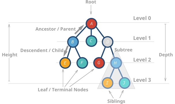
Here are some properties of trees:
- The top-most node is called root.
- A node without children is called leaf node or terminal node.
- Height (h) of the tree is the distance (edge count) between the farthest leaf to the root.
Ahas a height of 3Ihas a height of 0
- Depth or level of a node is the distance between the root and the node in question.
Hhas a depth of 2Bhas a depth of 1
Implementing a simple tree data structure
As we saw earlier, a tree node is just a data structure with a value and links to its descendants.
Here’s an example of a tree node:
1 | class TreeNode { |
We can create a tree with 3 descendants as follows:
1 | // create nodes with values |
That’s all; we have a tree data structure!
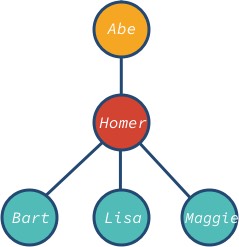
The node abe is the root and bart, lisa and maggie are the leaf nodes of the tree. Notice that the tree’s node can have different descendants: 0, 1, 3, or any other value.
Tree data structures have many applications such as:
- Maps
- Sets
- Databases
- Priority Queues
- Querying an LDAP (Lightweight Directory Access Protocol)
- Representing the Document Object Model (DOM) for HTML on Websites.
Binary Trees
Trees nodes can have zero or more children. However, when a tree has at the most two children, then it’s called binary tree.
Full, Complete, and Perfect binary trees
Depending on how nodes are arranged in a binary tree, it can be full, complete and perfect:
- Full binary tree: each node has exactly 0 or 2 children (but never 1).
- Complete binary tree: when all levels except the last one are full with nodes.
- Perfect binary tree: when all the levels (including the last one) are full of nodes.
Look at these examples:

These properties are not always mutually exclusive. You can have more than one:
- A perfect tree is always complete and full.
- Perfect binary trees have precisely nodes, where
kis the last level of the tree (starting with 1).
- Perfect binary trees have precisely nodes, where
- A complete tree is not always
full.- Like in our “complete” example, since it has a parent with only one child. If we remove the rightmost gray node, then we would have a complete and full tree but not perfect.
- A full tree is not always complete and perfect.
Binary Search Tree (BST)
Binary Search Trees or BST for short are a particular application of binary trees. BST has at most two nodes (like all binary trees). However, the values are so that the left children value must be less than the parent, and the right children must be higher.
Duplicates: Some BST doesn’t allow duplicates while others add the same values as a right child. Other implementations might keep a count on a case of duplicity (we are going to do this one later).
Let’s implement a Binary Search Tree!
BST Implementation
BST are very similar to our previous implementation of a tree. However, there are some differences:
- Nodes can have, at most, only two children: left and right.
- Nodes values has to be ordered as
left < parent < right.
Here’s the tree node. Very similar to what we did before, but we added some handy getters and setters for left and right children. Notice is also keeping a reference to the parent, and we update it every time we add children.
1 | const LEFT = 0; |
Ok, so far, we can add a left and right child. Now, let’s do the BST class that enforces the left < parent < right rule.
1 |
|
Let’s implementing insertion.
BST Node Insertion
To insert a node in a binary tree, we do the following:
- If a tree is empty, the first node becomes the root, and you are done.
- Compare root/parent’s value if it’s higher go right, if it’s lower go left. If it’s the same, then the value already exists so that you can increase the duplicate count (multiplicity).
- Repeat #2 until we found an empty slot to insert the new node.
Let’s do an illustration how to insert 30, 40, 10, 15, 12, 50:

We can implement insert as follows:
1 | add(value) { |
We are using a helper function called findNodeAndParent. If we found that the node already exists in the tree, then we increase the multiplicity counter. Let’s see how this function is implemented:
1 | findNodeAndParent(value) { |
findNodeAndParent goes through the tree, searching for the value. It starts at the root (line 2) and then goes left or right based on the value (line 10). If the value already exists, it will return the node found and also the parent. In case that the node doesn’t exist, we still return the parent.
BST Node Deletion
We know how to insert and search for value. Now, we are going to implement the delete operation. It’s a little trickier than adding, so let’s explain it with the following cases:
Deleting a leaf node (0 children)
1 | 30 30 |
We remove the reference from the node’s parent (15) to be null.
Deleting a node with one child.
1 | 30 30 |
In this case, we go to the parent (30) and replace the child (10) with a child’s child (15).
Deleting a node with two children
1 | 30 30 |
We are removing node 40, which has two children (35 and 50). We replace the parent’s (30) child (40) with the child’s right child (50). Then we keep the left child (35) in the same place before, so we have to make it the left child of 50.
Another way to remove node 40 is to move the left child (35) up and then keep the right child (50) where it was.
1 | 30 |
Either way is ok as long as you keep the binary search tree property: left < parent < right.
Deleting the root.
1 | 30* 50 |
Deleting the root is very similar to removing nodes with 0, 1, or 2 children discussed earlier. The only difference is that afterward, we need to update the reference of the root of the tree.
Here’s an animation of what we discussed.
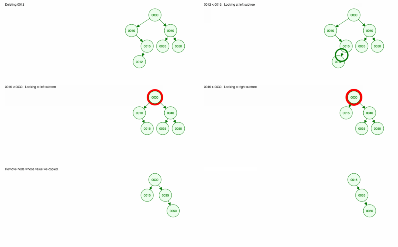
The animation moves up the left child/subtree and keeps the right child/subtree in place.
Now that we have a good idea how it should work, let’s implement it:
1 | remove(value) { |
Here are some highlights of the implementation:
- First, we search if the node exists. If it doesn’t, we return false, and we are done!
- If the node to remove exists, then combine left and right children into one subtree.
- Replace node to delete with the combined subtree.
The function that combines left into right subtree is the following:
1 | combineLeftIntoRightSubtree(node) { |
For instance, let’s say that we want to combine the following tree, and we are about to delete node 30. We want to mix the 30’s left subtree into the right one. The result is this:
1 | 30* 40 |
If we make the new subtree the root, then node 30 is no more!
Binary Tree Transversal
There are different ways of traversing a Binary Tree, depending on the order that the nodes are visited: in-order, pre-order, and post-order. Also, we can use them DFS and BFS that we learned from the graph post. Let’s go through each one.
In-Order Traversal
In-order traversal visit nodes on this order: left, parent, right.
1 | * inOrderTraversal(node = this.root) { |
Let’s use this tree to make the example:
1 | 10 |
In-order traversal would print out the following values: 3, 4, 5, 10, 15, 30, 40. If the tree is a BST, then the nodes will be sorted in ascendent order as in our example.
Post-Order Traversal
Post-order traversal visit nodes on this order: left, right, parent.
1 | * postOrderTraversal(node = this.root) { |
Post-order traversal would print out the following values: 3, 4, 5, 15, 40, 30, 10.
Pre-Order Traversal and DFS
Pre-order traversal visit nodes on this order: parent, left, right.
1 | * preOrderTraversal(node = this.root) { |
Pre-order traversal would print out the following values: 10, 5, 4, 3, 30, 15, 40. This order of numbers is the same result that we would get if we run the Depth-First Search (DFS).
1 | * dfs() { |
If you need a refresher on DFS, we covered it in detail on Graph post.
Breadth-First Search (BFS)
Similar to DFS, we can implement a BFS by switching the Stack by a Queue:
1 | * bfs() { |
The BFS order is: 10, 5, 30, 4, 15, 40, 3
Balanced vs. Non-balanced Trees
So far, we have discussed how to add, remove, and find elements. However, we haven’t talked about runtimes. Let’s think about the worst-case scenarios.
Let’s say that we want to add numbers in ascending order.

We will end up with all the nodes on the right side! This unbalanced tree is no better than a LinkedList, so finding an element would take O(n). 😱
Looking for something in an unbalanced tree is like looking for a word in the dictionary page by page. When the tree is balanced, you can open the dictionary in the middle, and from there, you know if you have to go left or right depending on the alphabet and the word you are looking for.
We need to find a way to balance the tree!
If the tree was balanced, we could find elements in O(log n) instead of going through each node. Let’s talk about what a balanced tree means.
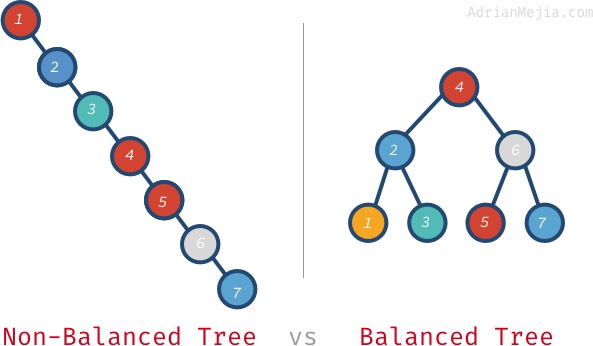
If we search for 7 in the non-balanced tree, we have to go from 1 to 7. However, in the balanced tree, we visit: 4, 6, and 7. It gets even worse with larger trees. If you have one million nodes, searching for a non-existing element might require you to visit all million while on a balanced tree. It just needs 20 visits! That’s a huge difference!
We are going to solve this issue in the next post using self-balanced trees (AVL trees).
Summary
We have covered much ground for trees. Let’s sum it up with bullets:
- The tree is a data structure where a node has 0 or more descendants/children.
- Tree nodes don’t have cycles (acyclic). If it has cycles, it is a Graph data structure instead.
- Trees with two children or less are called: Binary Tree
- When a Binary Tree is sorted so that the left value is less than the parent and the right children is higher, then and only then we have a Binary Search Tree.
- You can visit a tree in a pre/post/in-order fashion.
- An unbalanced has a time complexity of O(n). 🤦🏻
- A balanced has a time complexity of O(log n). 🎉

