Finding out the time complexity of your code can help you develop better programs that run faster. Some functions are easy to analyze, but when you have loops, and recursion might get a little trickier when you have recursion. After reading this post, you are able to derive the time complexity of any code.
In general, you can determine the time complexity by analyzing the program’s statements (go line by line). However, you have to be mindful how are the statements arranged. Suppose they are inside a loop or have function calls or even recursion. All these factors affect the runtime of your code. Let’s see how to deal with these cases.
Big O Notation
How to calculate time complexity of any algorithm or program? The most common metric it’s using Big O notation.
Here are some highlights about Big O Notation:
- Big O notation is a framework to analyze and compare algorithms.
- Amount of work the CPU has to do (time complexity) as the input size grows (towards infinity).
- Big O = Big Order function. Drop constants and lower order terms. E.g.
O(3*n^2 + 10n + 10)becomesO(n^2). - Big O notation cares about the worst-case scenario. E.g., when you want to sort and elements in the array are in reverse order for some sorting algorithms.
For instance, if you have a function that takes an array as an input, if you increase the number of elements in the collection, you still perform the same operations; you have a constant runtime. On the other hand, if the CPU’s work grows proportionally to the input array size, you have a linear runtime O(n).
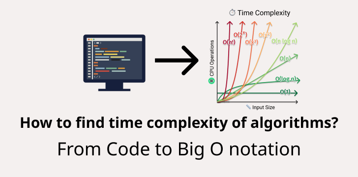
If we plot the most common Big O notation examples, we would have graph like this:

As you can see, you want to lower the time complexity function to have better performance.
Let’s take a look, how do we translate code into time complexity.
Sequential Statements
If we have statements with basic operations like comparisons, assignments, reading a variable.
We can assume they take constant time each O(1).
1 | statement1; |
If we calculate the total time complexity, it would be something like this:
1 | total = time(statement1) + time(statement2) + ... time (statementN) |
Let’s use T(n) as the total time in function of the input size n, and t as the time complexity taken by a statement or group of statements.
1 | T(n) = t(statement1) + t(statement2) + ... + t(statementN); |
If each statement executes a basic operation, we can say it takes constant time O(1). As long as you have a fixed number of operations, it will be constant time, even if we have 1 or 100 of these statements.
Example:
Let’s say we can compute the square sum of 3 numbers.
1 | function squareSum(a, b, c) { |
As you can see, each statement is a basic operation (math and assignment). Each line takes constant time O(1). If we add up all statements’ time it will still be O(1). It doesn’t matter if the numbers are 0 or 9,007,199,254,740,991, it will perform the same number of operations.
⚠️ Be careful with function calls. You will have to go to the implementation and check their run time. More on that later.
Conditional Statements
Very rarely, you have a code without any conditional statement. How do you calculate the time complexity? Remember that we care about the worst-case with Big O so that we will take the maximum possible runtime.
1 | if (isValid) { |
Since we are after the worst-case we take whichever is larger:
1 | T(n) = Math.max([t(statement1) + t(statement2)], [time(statement3)]) |
Example:
1 | if (isValid) { |
What’s the runtime? The if block has a runtime of O(n log n) (that’s common runtime for efficient sorting algorithms). The else block has a runtime of O(1).
So we have the following:
1 | O([n log n] + [n]) => O(n log n) |
Since n log n has a higher order than n, we can express the time complexity as O(n log n).
Loop Statements
Another prevalent scenario is loops like for-loops or while-loops.
Linear Time Loops
For any loop, we find out the runtime of the block inside them and multiply it by the number of times the program will repeat the loop.
1 | for (let i = 0; i < array.length; i++) { |
For this example, the loop is executed array.length, assuming n is the length of the array, we get the following:
1 | T(n) = n * [ t(statement1) + t(statement2) ] |
All loops that grow proportionally to the input size have a linear time complexity O(n). If you loop through only half of the array, that’s still O(n). Remember that we drop the constants so 1/2 n => O(n).
Constant-Time Loops
However, if a constant number bounds the loop, let’s say 4 (or even 400). Then, the runtime is constant O(4) -> O(1). See the following example.
1 | for (let i = 0; i < 4; i++) { |
That code is O(1) because it no longer depends on the input size. It will always run statement 1 and 2 four times.
Logarithmic Time Loops
Consider the following code, where we divide an array in half on each iteration (binary search):
1 | function fn1(array, target, low = 0, high = array.length - 1) { |
This function divides the array by its middle point on each iteration. The while loop will execute the amount of times that we can divide array.length in half. We can calculate this using the log function.
E.g. If the array’s length is 8, then we the while loop will execute 3 times because log2(8) = 3.
Nested loops statements
Sometimes you might need to visit all the elements on a 2D array (grid/table). For such cases, you might find yourself with two nested loops.
1 | for (let i = 0; i < n; i++) { |
For this case, you would have something like this:
1 | T(n) = n * [t(statement1) + m * t(statement2...3)] |
Assuming the statements from 1 to 3 are O(1), we would have a runtime of O(n * m).
If instead of m, you had to iterate on n again, then it would be O(n^2). Another typical case is having a function inside a loop. Let’s see how to deal with that next.
Function call statements
When you calculate your programs’ time complexity and invoke a function, you need to be aware of its runtime. If you created the function, that might be a simple inspection of the implementation. If you are using a library function, you might need to check out the language/library documentation or source code.
Let’s say you have the following program:
1 | for (let i = 0; i < n; i++) { |
Depending on the runtime of fn1, fn2, and fn3, you would have different runtimes.
- If they all are constant
O(1), then the final runtime would beO(n^3). - However, if only
fn1andfn2are constant andfn3has a runtime ofO(n^2), this program will have a runtime ofO(n^5). Another way to look at it is, iffn3has two nested and you replace the invocation with the actual implementation, you would have five nested loops.
In general, you will have something like this:
1 | T(n) = n * [ t(fn1()) + n * [ t(fn2()) + n * [ t(fn3()) ] ] ] |
Recursive Functions Statements
Analyzing the runtime of recursive functions might get a little tricky. There are different ways to do it. One intuitive way is to explore the recursion tree.
Let’s say that we have the following program:
1 | function fn(n) { |
You can represent each function invocation as a bubble (or node).
Let’s do some examples:
- When you n = 2, you have 3 function calls. First
fn(2)which in turn callsfn(1)andfn(0). - For
n = 3, you have 5 function calls. Firstfn(3), which in turn callsfn(2)andfn(1)and so on. - For
n = 4, you have 9 function calls. Firstfn(4), which in turn callsfn(3)andfn(2)and so on.
Since it’s a binary tree, we can sense that every time n increases by one, we would have to perform at most the double of operations.
Here’s the graphical representation of the 3 examples:

If you take a look at the generated tree calls, the leftmost nodes go down in descending order: fn(4), fn(3), fn(2), fn(1), which means that the height of the tree (or the number of levels) on the tree will be n.
The total number of calls, in a complete binary tree, is 2^n - 1. As you can see in fn(4), the tree is not complete. The last level will only have two nodes, fn(1) and fn(0), while a complete tree would have 8 nodes. But still, we can say the runtime would be exponential O(2^n). It won’t get any worst because 2^n is the upper bound.
Summary
In this chapter, we learned how to calculate the time complexity of our code when we have the following elements:
- Basic operations like assignments, bit, and math operators.
- Loops and nested loops
- Function invocations and recursions.
If you want to see more code examples for O(n log n), O(n^2), O(n!), check out the most common time complexities that every developer should know.