In this post, we are going to explore non-linear data structures like graphs. Also, we’ll cover the central concepts and typical applications.
You are probably using programs with graphs and trees. For instance, let’s say that you want to know the shortest path between your workplace and home. You can use graph algorithms to get the answer! We are going to look into this and other fun challenges.
In the previous post, we explore linear data structures like arrays, linked lists, sets, stacks, etc. This one builds on top of what we learned.
You can find all these implementations and more in the Github repo: https://github.com/amejiarosario/dsa.js
This post is part of a tutorial series:
Learning Data Structures and Algorithms (DSA) for Beginners
Graph Data Structures for Beginners 👈 you are here
Here is the summary of the operations that we are going to cover on this post:
| Adjacency List | Adjacency Matrix | |
|---|---|---|
| Space | O(|V| + |E|) | O(|V|2) |
| addVertex | O(1) | O(|V|2) |
| removeVertex | O(|V| + |E|) | O(|V|2) |
| addEdge | O(1) | O(1) |
| removeEdge (using Array) | O(|E|) | O(1) |
| removeEdge (using HashSet) | O(1) | O(1) |
| getAdjacents | O(|E|) | O(|V|) |
| isAdjacent (using Array) | O(|E|) | O(1) |
| isAdjacent (using HashSet) | O(1) | O(1) |
Graphs Basics
Before we dive into interesting graph algorithms, let’s first clarify the naming conventions and graph properties.
A graph is a data structure where a node can have zero or more adjacent elements.
The connection between two nodes is called edge. Nodes can also be called vertices.
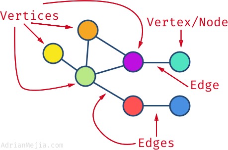
The degree is the number of edges connected to a vertex. E.g., the purple vertex has a degree of 3 while the blue one has a degree of 1.
If the edges are bi-directional, then we have an undirected graph. If the edges have a direction, then we have a directed graph or di-graph for short. You can think of it as a one-way street (directed) or two-way street (undirected).
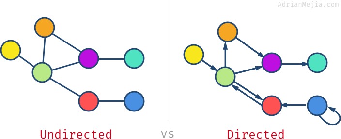
Vertex can have edges that go to itself (e.g., blue node). This is called self-loop.
A graph can have cycles, which means you could get the same node more than once. The graph without cycles is called acyclic graph.
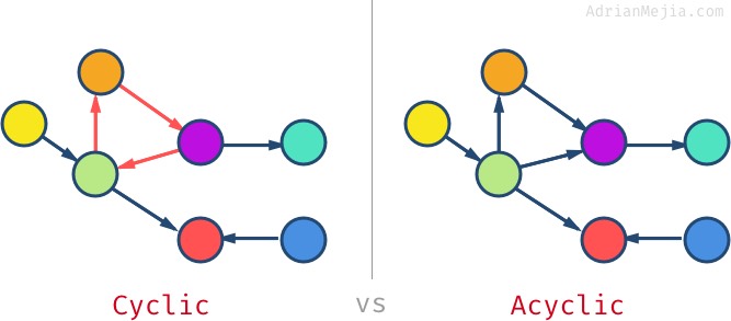
Also, acyclic undirected graphs are called tree. We are going to cover trees in-depth in the next post.
Not all vertices have to be connected in the graph. You might have isolated nodes or even separated subgraphs. If all nodes have at least one edge, then we have a connected graph. When all nodes are connected to all other nodes, then we have a complete graph.
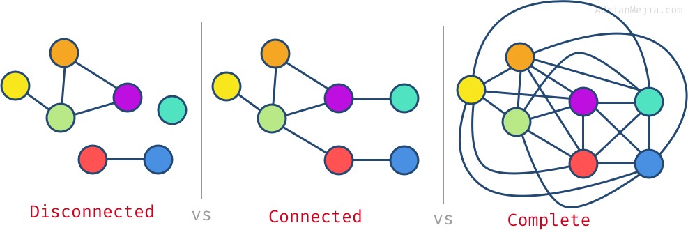
For a complete graph, each node should have #nodes - 1 edges. In the previous example, we have seven vertices, so each node has six edges.
Graph Applications
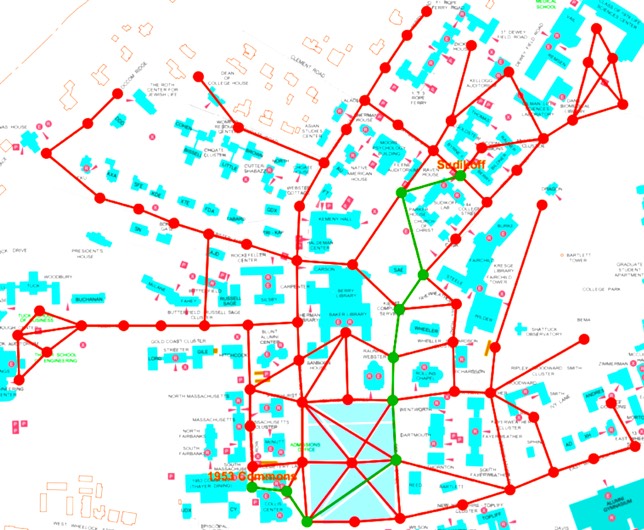
When edges have values/cost assigned to them, we say we have a weighted graph. If the weight is absent, we can assume it’s 1.

Weighted graphs have many applications depending on the domain where you need to solve a problem. To name a few:
Airline Traffic (image above)
- Node/vertex = Airport
- Edges = direct flights between two airports
- Weight = miles between two airports
GPS Navigation
- Node = road intersection
- Edge = road
- Weight = time required to go from one intersection to another
Networks routing
- Node = server
- Edge = data link
- Weight = connection speed
In general, graphs have many real-world applications like:
- Electronic circuits
- Flight reservations
- Driving directions
- Telcom: Cell tower frequency planning
- Social networks. E.g., Facebook uses a graph for suggesting friends
- Recommendations: Amazon/Netflix uses graphs to make suggestions for products/movies
- Graphs help to plan the logistics of delivering goods
We just learned the basics of graphs and some applications. Let’s cover how to represent graphs in JavaScript.
Representing graphs
There are two primary ways of representing a graph:
- Adjacency list
- Adjacency Matrix
Let’s explain it with the following directed graph (digraph) as an example:
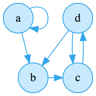
We digraph with 4 nodes. When a vertex has a link to itself (e.g. a) is called self-loop.
Adjacency Matrix
The adjacency matrix is one way of representing a graph using a two-dimensional array (NxN matrix). In the intersection of nodes, we add 1 (or other weight) if they are connected and 0 or - if they are not connected.
Using the same example as before, we can build the following adjacency matrix:
1 | a b c d e |
As you can see, the matrix list all nodes horizontally and vertically. If there are a few connections, we call it a sparse graph. If there are many connections (close to the max number of links), we call it a dense graph. If all possible connections are reached, then we have a complete graph.
It’s important to notice that the adjacency matrix will always be symmetrical by the diagonal for undirected graphs. However, that’s not always the case on a digraph (like our example).
What is the time complexity of finding connections of two vertices?
Querying if two nodes are connected in an adjacency matrix takes a constant time or O(1).
What is the space complexity?
Storing a graph as an adjacency matrix has a space complexity of O(n2), where
nis the number of vertices. Also, represented as O(|V|2)
What is the runtime to add a vertex?
The vertices are stored as a VxV matrix. So, every time a vertex is added, the matrix needs to be reconstructed to a V+1xV+1.
Adding a vertex on an adjacency matrix is O(|V|2)
What about getting the adjacent nodes?
Since the matrix has a VxV matrix, we would have to go to the node row to get all the adjacent nodes to a given vertex and get all its edges with the other nodes.
In our previous example, let’s say we want all the adjacent nodes to b. We have to get the full row where b is with all the other nodes.
1 | a b c d e |
We have to visit all nodes so,
Getting adjacent nodes on an adjacency matrix is O(|V|)
Imagine that you need to represent the Facebook network as a graph. You would have to create a matrix of 2 billion x 2 billion, where most of it would be empty! Nobody would know everybody else, just a few thousand at most.
In general, we deal with sparse graphs so that the matrix will waste a lot of space. That’s why, in most implementations, we would use an adjacency list rather than the matrix.
Adjacency List
Adjacency List is one of the most common ways to represent graphs. Each node has a list of all the nodes connected to it.
Graphs can be represented as an adjacency list using an Array (or HashMap) containing the nodes. Each node includes a list (Array, linked list, set, etc.) that lists its adjacent nodes.
For instance, in the graph above we have that a has a connection to b and also a self-loop to itself. In turn, b has a connection to c and so on:
1 | a -> { a b } |
As you can imagine, if you want to know if a node is connected to another node, you would have to go through the list.
Querying if two nodes are connected in an adjacency list is O(n), where
nis the number of vertices. Also represented as O(|V|)
What about space complexity?
Storing a graph as an adjacency list has a space complexity of O(n), where
nis the sum of vertices and edges. Also, represented as O(|V| + |E|)
Adjacency List Graph HashMap Implementation
The adjacency list is the most common way of representing graphs. There are several ways to implement the adjacency list:
One of them is using a HashMap. The key is the node’s value, and the value is an array of adjacency.
1 | const graph = { |
Graph usually needs the following operations:
- Add and remove vertices
- Add and remove edges
Adding and removing vertices involves updating the adjacency list.
Let’s say that we want to remove the vertex b. We could do delete graph['b'];. However, we still have to remove the references on the adjacency list on d and a.
Every time we remove a node, we would have to iterate through all the nodes’ list O(|V| + |E|). Can we do better? We will answer that soon, but first, let’s *implement our list in a more object-oriented way to swap implementations easily.
Adjacency List Graph OO Implementation
Let’s start with the Node class that holds the vertex’s value and adjacent vertices. We can also have helper functions for adding and removing adjacent nodes from the list.
1 | class Node { |
Notice that adjacent runtime is O(1), while remove adjacent is O(|E|). What if, instead of an array, use a HashSet 🧐? It could be O(1). But, let first get it working, and later we can make it faster.
Make it work. Make it right. Make it faster.
Ok, now that we have the Node class, let’s build the Graph class to perform operations such as adding/removing vertices and edges.
Graph.constructor
1 | class Graph { |
The first thing that we need to know is if the graph is directed or undirected. That makes a difference when we are adding edges.
Graph.addEdge
To add an edge, we need two nodes. One is the source, and the other is the destination.
1 | addEdge(source, destination) { |
We add an edge from the source vertex to the destination. If we have an undirected graph, we also add from target node to source since it’s bidirectional.
The runtime of adding an edge from a graph adjacency list is: O(1)
If we try to add an edge and the nodes don’t exist, we need to create them first. Let’s do that next!
Graph.addVertex
The way we create a node is that we add it to the this.nodes Map. The map store a key/value pair, where the key is the vertex’s value while the map value is the instance of the node class. Take a look at line 5-6:
1 | addVertex(value) { |
If the node already exists, we don’t want to overwrite it. So, we first check if it already exists, and if it doesn’t, then we create it.
The runtime of adding a vertex from a graph adjacency list is: O(1)
Graph.removeVertex
Removing a node from the graph, it’s a little bit more involved. We have to check if the node to be deleted it’s in use as an adjacent node.
1 | removeVertex(value) { |
We have to go through each vertex and then each adjacent node (edges).
The runtime of removing a vertex from a graph adjacency list is O(|V| + |E|)
Finally, let’s remove implement removing an edge!
Graph.removeEdge
Removing an edge is pretty straightforward and similar to addEdge.
1 | removeEdge(source, destination) { |
The main difference between addEdge and removeEdge is that:
- If the vertices don’t exist, we won’t create them.
- We use
Node.removeAdjacentinstead ofNode.addAdjacent.
Since removeAdjacent has to go through all the adjacent vertices, we have the following runtime:
The runtime of removing an edge from a graph adjacency list is O(|E|)
We are going to explore how to search for values from a node.
Breadth-first search (BFS) - Graph search
Breadth-first search is a way to navigate a graph from an initial vertex by visiting all the adjacent nodes first.
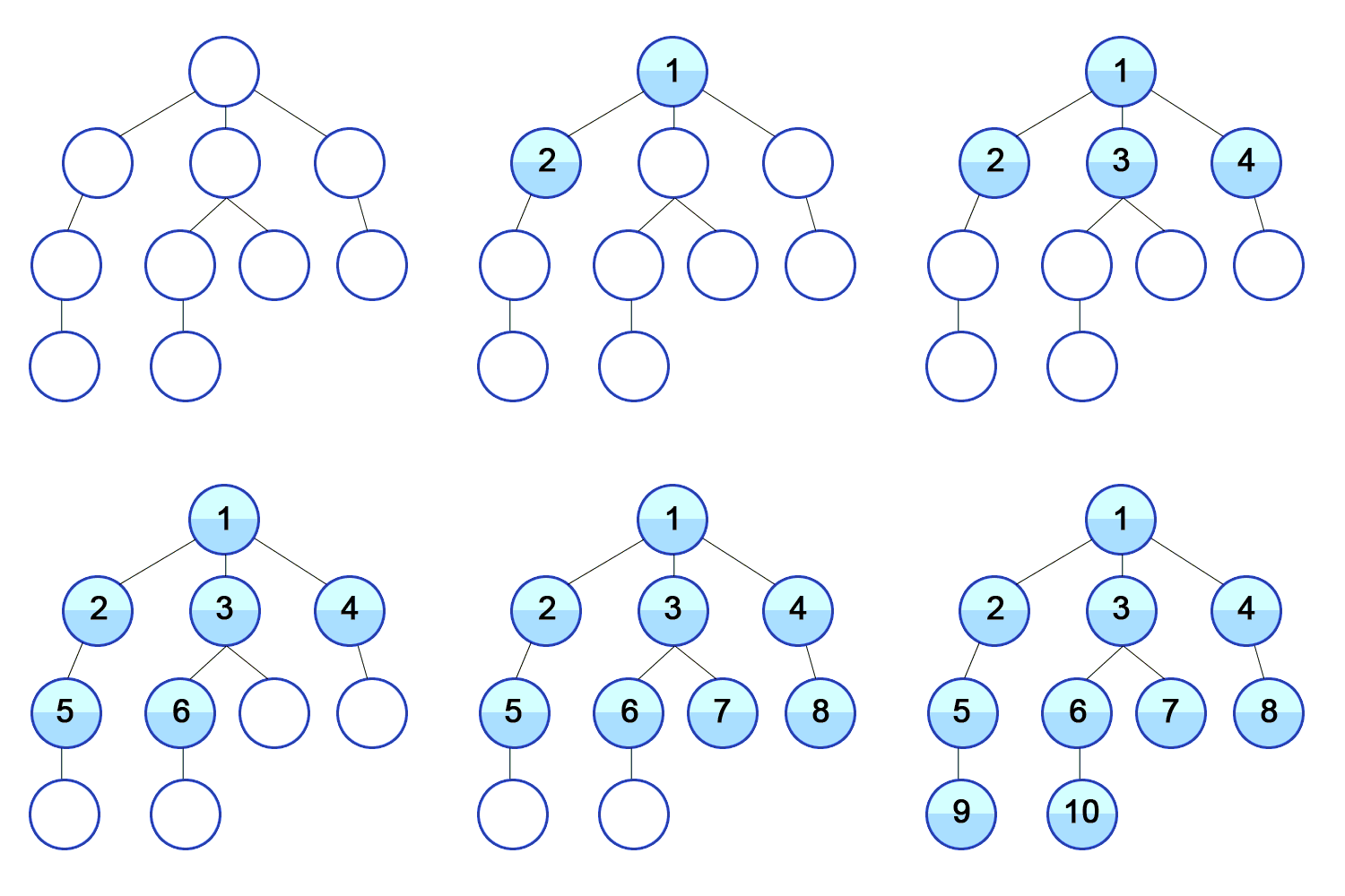
Let’s see how we can accomplish this in code:
1 | *bfs(first) { |
As you can see, we are using a Queue where the first node is also the first node to be visited (FIFO). You can find the Queue implementation here.
We are using JavaScript generators, notice the * in front of the function. This generator iterates one value at a time. That’s useful for large graphs (millions of nodes) because you don’t need to visit every single node in most cases.
This an example of how to use the BFS that we just created:
1 | const graph = new Graph(Graph.UNDIRECTED); |
You can find more illustrations of usage in the test cases. Let’s move on to the DFS!
Depth-first search (DFS) - Graph search
Depth-first search is another way to navigate a graph from an initial vertex by recursively the first adjacent node of each vertex found.

The iterative implementation of a DFS is identical to the BFS, but instead of using a Queue you use a Stack:
NOTE: stack implementation
1 | *dfs(first) { |
We can test our graph as follow.
1 | const graph = new Graph(Graph.UNDIRECTED); |
As you can see, the graph is the same on BFS and DFS. However, the order of how the nodes were visited is very different. BFS went from 1 to 10 in that order, while DFS went as deep as it could on each node.
Graph Time and Space Complexity
We have seen some of the basic operations of a Graph. How to add and remove vertices and edges. Here’s a summary of what we have covered so far:
| Adjacency List | Adjacency Matrix | |
|---|---|---|
| Space | O(|V| + |E|) | O(|V|2) |
| addVertex | O(1) | O(|V|2) |
| removeVertex | O(|V| + |E|) | O(|V|2) |
| addEdge | O(1) | O(1) |
| removeEdge (using Array) | O(|E|) | O(1) |
| removeEdge (using HashSet) | O(1) | O(1) |
| getAdjacents | O(|E|) | O(|V|) |
| isAdjacent (using Array) | O(|E|) | O(1) |
| isAdjacent (using HashSet) | O(1) | O(1) |
As you can see, an adjacency list is faster in almost all operations. The only action that the adjacency matrix will outperform the adjacency list is checking if a node is adjacent to another. However, if we change our implementation from Array to a HashSet, we can get it in constant time.
Summary
As we saw, Graphs can help to model many real-life scenarios such as airports, social networks, the internet, and so on. We covered some of the most fundamental algorithms, such as Breadth-First Search (BFS) and Depth-First Search (DFS). Also, we studied implementation trade-offs such as adjacency lists and matrix. Subscribe to my newsletter and don’t miss any of my posts because there are many other applications that we will learn soon, such as finding the shortest path between nodes and different exciting graph algorithms!

