As a developer, you have the power to change the world! You can write programs that enable new technologies. For instance, develop software to find an earlier diagnosis of diseases. But that’s not the only way. You might do it indirectly by creating projects that make people more productive and help them free up time to do other amazing things. Whatever you do, it has the potential to impact the community who use it.
However, these accomplishments are only possible if we write software that is fast and can scale. Learning how to measure your code performance is the goal of this post.
This post is part of a tutorial series:
Learning Data Structures and Algorithms (DSA) for Beginners
Intro to Algorithm’s Time Complexity and Big O Notation 👈 you are here
We will explore how you can measure your code performance using analysis of algorithms: time complexity and big O notation.
First, let’s see a real story to learn why this is important.
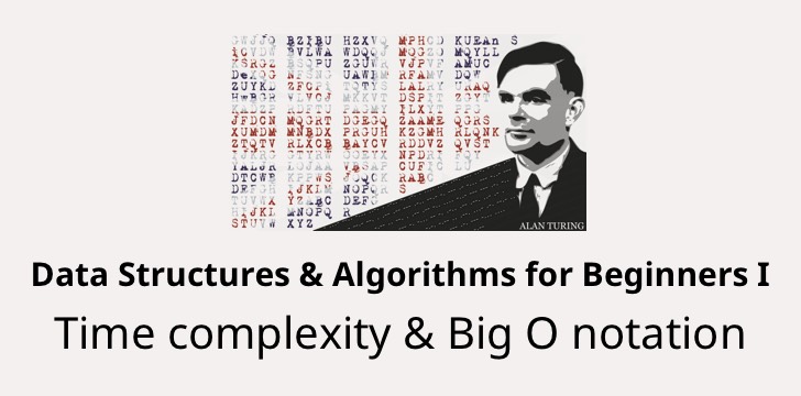
An algorithm that saved millions of lives
During World War II, the Germans used AM radio signals to communicate with troops around Europe. Anybody with an AM frequency radio and some knowledge of Morse code could intercept the message. However, the information was encoded! All the countries that were under attack tried to decode it. Sometimes, they got lucky and could make sense of a couple of messages at the end of the day. Unfortunately, the Nazis changed the encoding every single day!
A brilliant mathematician called Alan Turing joined the British military to crack the German “Enigma” code. He knew they would never get ahead if they keep doing the calculations by pen and paper. So after many months of hard work, they built a machine. Unfortunately, the first version of the device took too long to decode a message! So, it was not very useful.
Alan’s team found out that every encrypted message ended with the same string: “Heil Hitler” Aha! After changing the algorithm, the machine was able to decode transmissions a lot faster! They used the info to finish the war quicker and save millions of lives!
The same machine that was going to get shut down as a failure became a live saver. Likewise, you can do way more with your computing resources when you write efficient code. That is what we are going to learn in this post series!
Another popular algorithm is PageRank developed in 1998 by Sergey Brin and Larry Page (Google founders). This algorithm was (and is) used by a Google search engine to make sense of trillions of web pages. Google was not the only search engine. However, since their algorithm returned better results, most of the competitors faded away. Today it powers most of 3 billion daily searches very quickly. That is the power of algorithms that scale! 🏋🏻
So, why should you learn to write efficient algorithms?
There are many advantages; these are just some of them:
- You would become a much better software developer (and get better jobs/income).
- Spend less time debugging, optimizing, and re-writing code.
- Your software will run faster with the same hardware (cheaper to scale).
- Your programs might be used to aid discoveries that save lives (maybe?).
Without further ado, let’s step up our game!
What are algorithms?
Algorithms (as you might know) are steps of how to do some task. For example, when you cook, you follow a recipe to prepare a dish. If you play a game, you are devising strategies to help you win. Likewise, algorithms in computers are a set of instructions used to solve a problem.
Algorithms are instructions to perform a task
There are “good” and “bad” algorithms. The good ones are fast; the bad ones are slow. Slow algorithms cost more money and make some calculations impossible in our lifespan!
We are going to explore the basic concepts of algorithms. Also, we are going to learn how to distinguish “fast” from “slow” ones. Even better, you will be able to “measure” your algorithms’ performance and improve them!
How to improve your coding skills?
The first step to improving something is to measure it.
Measurement is the first step that leads to control and eventually to improvement. If you can’t measure something, you can’t understand it. If you can’t understand it, you can’t control it. If you can’t control it, you can’t improve it.
How do you do “measure” your code? Would you clock “how long” it takes to run? What if you are running the same program on a mobile device or a quantum computer? The same code will give you different results.
To answer these questions, we need to nail some concepts first, like time complexity!
Time complexity
Time complexity (or running time) is the estimated time an algorithm takes to run. However, you do not measure time complexity in seconds, but as a function of the input. (I know it’s weird but bear with me).
The time complexity is not about timing how long the algorithm takes. Instead, how many operations are executed. The number of instructions executed by a program is affected by the input’s size and how their elements are arranged.
Why is that the time complexity is expressed as a function of the input? Well, let’s say you want to sort an array of numbers. If the elements are already sorted, the program will perform fewer operations. On the contrary, if the items are in reverse order, it will require more time to get them sorted. The time a program takes to execute is directly related to the input size and its arrangement.
We can say for each algorithm have the following running times:
- Worst-case time complexity (e.g., input elements in reversed order)
- Best-case time complexity (e.g., already sorted)
- Average-case time complexity (e.g., elements in random order)
We usually care more about the worst-case time complexity (We hope for the best but preparing for the worst).
Calculating time complexity
Here’s a code example of how you can calculate the time complexity: Find the smallest number in an array.
1 | /** |
We can represent getMin as a function of the size of the input n based on the number of operations it has to perform. For simplicity, let’s assume that each line of code takes the same amount of time in the CPU to execute. Let’s make the sum:
- Line 6: 1 operation
- Line 7: 1 operation
- Line 9-13: it is a loop that executes
ntimes- Line 10: 1 operation
- Line 11: this one is tricky. It is inside a conditional. We will assume the worst case where the array is sorted in descending order. The condition (
ifblock) will be executed each time. Thus, one operation
- Line 14: 1 operation
All in all, we have 3 operations outside the loop and 2 inside the forEach block. Since the loop goes for the size of n, this leaves us with 2(n) + 3.
However, this expression is somewhat too specific, and hard to compare algorithms with it. We are going to apply the asymptotic analysis to simplify this expression further.
Asymptotic analysis
Asymptotic analysis is just evaluating functions as their value approximate to the infinite. In our previous example 2(n) + 3, we can generalize it as k(n) + c. As the value of n grows, the value c is less and less significant, as you can see in the following table:
| n (size) | operations | result |
|---|---|---|
| 1 | 2(1) + 3 | 5 |
| 10 | 2(10) + 3 | 23 |
| 100 | 2(100) + 3 | 203 |
| 1,000 | 2(1,000) + 3 | 2,003 |
| 10,000 | 2(10,000) + 3 | 20,003 |
Believe it or not, the constant k wouldn’t make too much of a difference. Using this kind of asymptotic analysis, we take the higher-order element, in this case: n.
Let’s do another example so we can get this concept. Let’s say we have the following function: `3 n^2 + 2n + 20`. What would be the result of using the asymptotic analysis?
`3 n^2 + 2n + 20` as `n` grows bigger and bigger; the term that will make the most difference is `n^2`.
Going back to our example, getMin, we can say that this function has a time complexity of n. As you can see, we could approximate it as 2(n) and drop the +3 since it does not add too much value as `n` keep getting bigger.
We are interested in the big picture here, and we are going to use the asymptotic analysis to help us with that. With this framework, comparing algorithms is much more comfortable. We can compare running times with their most crucial term: `n^2` or `n` or `2^n`.
Big-O notation and Growth rate of Functions
The Big O notation combines what we learned in the last two sections about worst-case time complexity and asymptotic analysis.
The letter `O` refers to the order of a function.
The Big O notation is used to classify algorithms by their worst running time. Also known as the upper bound of the growth rate of a function.
In our previous example with getMin function, we can say it has a running time of O(n). There are many different running times. Here are the most common that we are going to cover in the next post and their relationship with time:
Growth rates vs. n size:
| n | O(1) | O(log n) | O(n) | O(n log n) | O(n2) | O(2n) | O(n!) |
|---|---|---|---|---|---|---|---|
| 1 | < 1 sec | < 1 sec | < 1 sec | < 1 sec | < 1 sec | < 1 sec | < 1 sec |
| 10 | < 1 sec | < 1 sec | < 1 sec | < 1 sec | < 1 sec | < 1 sec | 4 sec |
| 100 | < 1 sec | < 1 sec | < 1 sec | < 1 sec | < 1 sec | 40170 trillion years | > vigintillion years |
| 1,000 | < 1 sec | < 1 sec | < 1 sec | < 1 sec | < 1 sec | > vigintillion years | > centillion years |
| 10,000 | < 1 sec | < 1 sec | < 1 sec | < 1 sec | 2 min | > centillion years | > centillion years |
| 100,000 | < 1 sec | < 1 sec | < 1 sec | 1 sec | 3 hours | > centillion years | > centillion years |
| 1,000,000 | < 1 sec | < 1 sec | 1 sec | 20 sec | 12 days | > centillion years | > centillion years |
As you can see, some algorithms are very time-consuming. It is impossible to compute an input size as little as 100 even if we had a supercomputer!! Hardware does not scale as well as software.
In the next post, we will explore all of these time complexities with a code example or two!
Are you ready to become a super programmer and scale your code?! ![]()
Continue with the next part 👉 Eight running times that every programmer should know